The Map of Triton

There is a cool video of Neptune’s moon Triton that NASA has put together using Voyager 2’s images:

io9 has a great article on how this was put together, plus a summary of what we know of Triton.

Sorting Out the Candidates

At this point, I have created rgb images for all the objects I want to check out in the field of view of interest. There were hundreds of objects, but that is why computer programming exists. So that they do all the hard work. Unfortunately, there are some things that machines aren’t that good at. So, as a human, my job is to look at these images and identify candidates. Brown dwarfs are dim in the visible and shiny in the infrared. So, my job is to look for dots that are like that. Take this picture, for example:

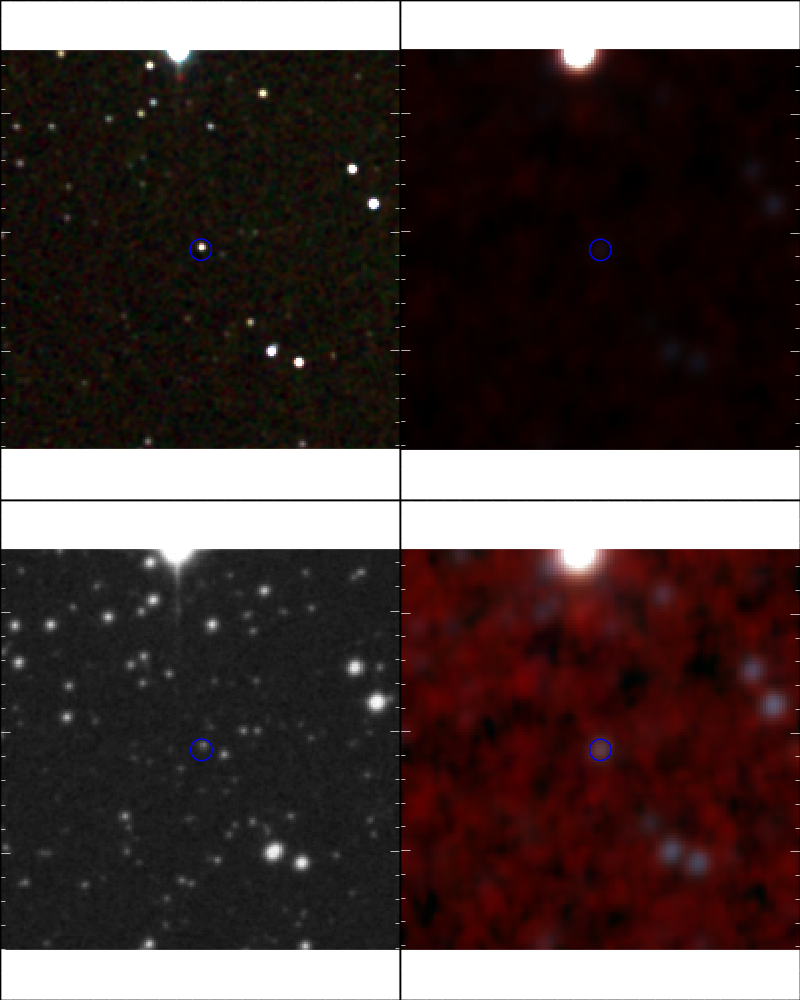
The bottom left one is from DSS Red, which was taken the earliest, around 1990 or so, the top left one is from 2MASS, which was taken around 2000, and the right ones are from WISE, taken around 2010. The top and bottom left only differ on how the colors are scaled in terms of brightness. The top left one is linear stretch, and the bottom left one is logarithmic stretch. As you can see, logarithmic stretch is very helpful because  with linear, the star on top is so bright that the other dots are comparatively almost nothing. With logarithmic stretch though, a star 10 times as bright can be treated as if it were only twice as bright, and 100 times as bright as if it were only three times as bright. This allows dim objects to pop out.

This one is of interest because you can observe proper motion here. Each one were taken around a decade apart, and as you can see, the dots have moved slightly. It suggests of an object relatively close. As to whether it is a brown dwarf, I am not sure, but I am keeping tabs on it just in case. It is something I am gonna have to discuss with the professor.

One RGB Image Using Three Images

This is an RGB image using the infrared bands of Wise 1, 2, and 3. These three images are of the same size, so it works on the astropy package I am using without having to install Montage. I made 3 red, 2 green, and 1 blue. As you can see from all that red smudge, WISE 3 is sort of hazier. You can’t actually see a brown dwarf very well from WISE 3 band, so I guess this helps.

Making Stars More Visible

Before I begin, there is a previous post that I would like to comment on my previous post. Apparently what I did was not combine three images and create an RGB image based on them. What happened instead was I put WISE 1, J, and K on top of each other, so all you could see was WISE 1 on top. Bummer. In order to do that, I have to install Montage, otherwise the images won’t rescale and stuff to fit each other. Unfortunately, it looks like a Linux kind of thing. Oh well.

Moving on to greener pastures, I have been changing a value called vmin and vmax. It allows me to set up a scale of color or black to white that depends on how bright the pixel is. So, let’s use the grayscale here for simplicity. If the pixel is as bright as the vmax value, then that pixel is white. If it is as dim as the vmin value, that pixel is black. In between it is all shades of gray. So, what happens, say if you bring the value of vmax down? The dimmer objects become whiter because now the brightness is closer to the vmax boundary. See here:

As you can see above, the bright object is still white when you lower the vmax boundary, but the whiteness becomes wider, while the dimmer object becomes whiter because it is closer to the line. That way, you can make dim objects stand out. See here two pictures below, one before the change, and one after:

As you can see, it is much clearer that there is actually a thing shining right in the middle of the circle. I made the brown dwarf stand out.

 

Meaning Science Museums Are Ran by a Bunch of Cowards

This is what it has come to. A bunch of science museums afraid of teaching facts about climate change because of moneyed interests not wanting their playtime to end. And the chickens running those places won’t even take a stand. Disgraceful.

In Which I Achieve Something

I made a colored picture using J band of 2MASS (1.25 micrometer), K band of 2MASS (2.17 micrometer), and Wise 1 (3.4 micrometer). Basically, each band represents the different wavelengths in which the telescopes captured the images. So, I put them together using python and got:

Neat! I believe the faint dot in the middle is the brown dwarf here. Hopefully I got did it right.

I Hope That Whoever Wrote the Programming Documentations Suffered Grievous Harm From Stepping on Legos

I spent hours upon hours trying to install APLpy with pip, trying whichever way to make it work. All because someone couldn’t give a damn about the details so it can be accessed by newcomers. So I am going to do everyone a favor and tell you all how to do this for Windows.

Installing pip itself is easy. Just follow the link, download it, and then double click on the python program. This will install pip by itself. It is the using part that made me want to rip my hair out. And according to a friend, it is kind of Windows fault for sucking so much. Anyways, firstly, turns out, don’t use the python shell. Use the command prompt. Yeah, they don’t tell you that, assuming your average newcomer is a giant computer nerd. Well, not everyone is a computer nerd, they can be a physics nerd like me, OKAY!

Next up, go to the PC icon, right click, properties, advanced system setting button, and go to the advanced tab. There is an option called “change environmental variable”. Click on PATH and edit it so it goes to C:\Python27(mine was python 2.7, yours might be different)\Scripts. NOW you can go to the command prompt and type: pip install name-of-package-from-PyPI-you-want-to-install.

I don’t know why that is and why this ridiculous roundabout way has to exist, but those goddamn writers didn’t even bother to make it easy for new users. They just tell you, “go do this” and expects you to automatically get what to do despite it not being obvious for noobs like me. Someone please hold a writing workshop or something for these people because I have just had it trying to install all these dependencies and making things work.

Planets of the Day: Kapteyn System and Kepler 10c

So, there have been two exciting planetary discoveries last week:

a) Two planets have been discovered around Kapteyn star, which is around 13 light years away. Since planets form with the star at around the same time, and the star is around 11.5 billion years old, the planets are the oldest known. Kapteyn star itself is likely to be a star of another tiny galaxy absorbed into the Milky Way, the remnant of that galaxy being the globular cluster Omega Centauri. Both planets are super Earth, with Kapteyn b having the possibility of liquid water to exist. Link here and here.

b) The most massive terrestrial planet yet has been discovered, and it is dubbed a mega Earth. Kepler 10c is 17 times the mass of the Earth, which is basically around Neptune’s mass. The size, though, is 2.3 times the Earth. This means the object has the density of a rock, so we know it can’t be a gas giant planet like Neptune. It is indeed a new type of planet, since a rocky planet is not expected to be this massive. I love surprises like this! More here and here.

I Got Sent More Reading Materials

I don’t have anything particular to say about them. They are pretty much a technical summary of brown dwarfs found, classification of spectra, proper motion (angle speed in sky), and distance, which were found using the 2MASS survey and WISE telescope. You can read them here, here, and here, if you want to learn more about brown dwarfs. They are pretty technical, though.

Update: You know what? I was mulling things over, and turns out there are a few things I want to comment about. Firstly, there is a spectral classification cooler than the T type, called the Y type, which is characterized by absorption from ammonia. These brown dwarfs are cooler than 600 K. The articles above talk about some of those.

Secondly, the articles above have a large focus on high proper motion brown dwarfs. Higher proper motion implies that the object are more probable to be closer to us than those having low proper motion. Think about it this way, when you are in a car, things that are far away look slower than things that are closer to you. It’s not so much that in reality things that are farther away are slower, as it is the fact that things that are farther away has lesser angular movement because distances look smaller when farther away.

How are proper motion found? Well, turns out that the 2MASS survey took observations a decade previous to WISE telescope. So, you look at the pictures from 2MASS, and you look at one from WISE, and see how much the position has changed in angle. The objects are likely to have constant speed, so just divide the angle difference by the year difference.

What is proper motion helpful for? Well, it let us know that an object is likely to be close to the solar system. This is supposed to help bridge the gap in our knowledge of the solar system neighborhood. The distance itself can later be taken using parallax. Aside from that, finding close brown dwarfs is also helpful because it will help us study the atmosphere better. We still have an imperfect model on the process behind condensation and cloud formation in the brown dwarf atmosphere, and the more of them we find, the better we will know the details behind it.

Brown Dwarf Pics

This is what an image for brown dwarf looks like, just a faint dot. As you can see in the link, each of those four images represent the different wavelength of infrared the pictures were taken. Obviously WISE band 1 and 2 (WISE is the name of the telescope) are best for this sort of stuff. Oh, and fun fact, this one was discovered by my prof.